A journey in the world of the Mathematics used in Computer Science.
Mathematics is used, a lot in Computer Science. In many fields like Computer Graphics, Data Science, Machine Learning, you'll need to use lots of Math. In this blog post, I'll mostly focus on Computer Graphics, which has many applications like Data Visualization, Video Games, Animations...
Computers have limitations
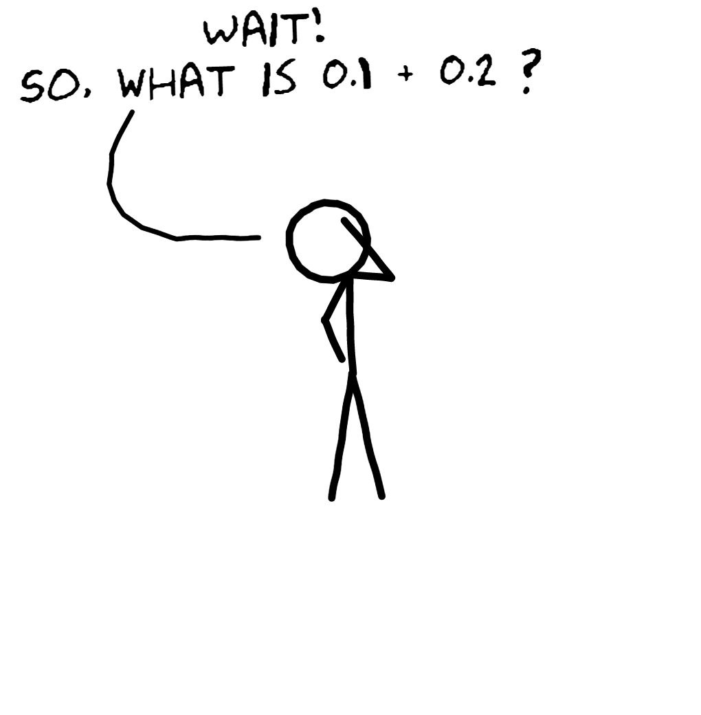
When working with a computer, you have a limited amount of memory. You can't store numbers with an infinite number of digits: for example, a computer thinks that $\pi$ has only 15 digits ($3.141592653589793$). This limited amount of precision can cause some problems with arithmetic like $0.1+0.2 \neq 0.3$
If you use Python, you can see:
>>> 0.1 + 0.2
0.30000000000000004
It's close, but it's not $0.3$. This isn't a problem with Python, it's a problem with every programming language that uses Floating Point arithmetic. We, as humans, have a similar problem: try to compute $\frac13+\frac23$ without using fractions' rules. If you use 10 digits to represent the two numbers, you have $0.3333333333 + 0.6666666666=0.9999999999$. But it's not precisely $1$.
In computer graphics, there is a similar problem. You have a screen with a limited amount of pixels.

In Computer Graphics, at some point, you need to draw lines. With vertical or horizontal lines, there are no problem: you set a row or a column of pixels to the specified color. However, with diagonal lines, it's trickier. You could do something like this:
This doesn't seem to be a line anymore, but it's as close as we can get. There isn't enough pixels to have a smooth line.
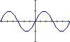
This is why, when you graph $y = \sin(x)$ on Desmos, you get a smooth curve. Whereas, on your calculator, it might have a more pixelated look.
So, how do you draw lines on screen with discrete pixels ? But first, we need to know how to draw points.
How to draw points on a screen ?
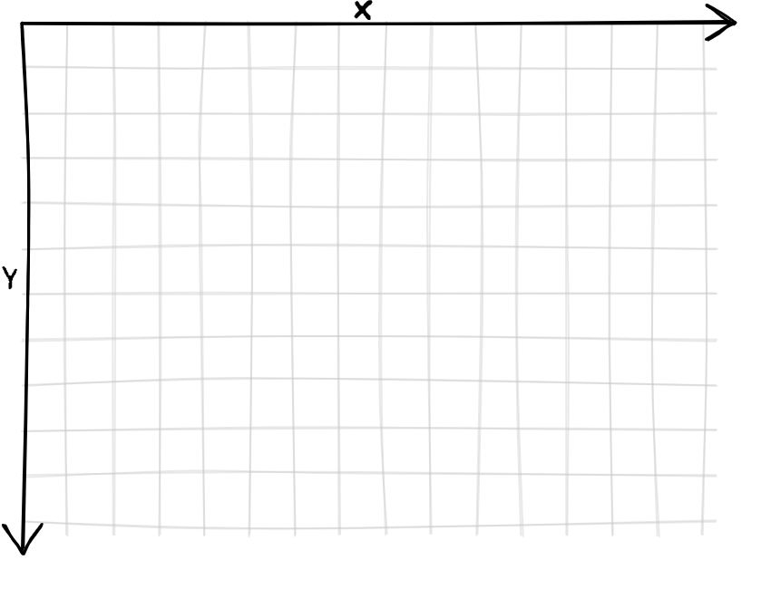
Usually, the screen uses a coordinate system where the origin is the top left point with the x-axis pointing to the right and the y-axis pointing down.
This coordinate system doesn't have the same orientation as what you're used to with function graphs with the y-axis pointing up.
If we need to draw a point at $(x,y)$ with $x$ and $y$ integers, it's easy. We just set the value of the pixel on the $y$th row and the $x$th column to the desired color.
If we want to plot points with non-integer coordinates (it'll be useful for later), it's also pretty easy. We just round the $x$ and $y$ coordinates to the nearest integer.
How do we implement it in code ?
# we will use 0 to represent black and 1 white
screen = [ [ 1 for x in range(height) ] for y in range(width) ]

def point(x, y):
    # we assume x and y are floats or ints

    if x < 0 or x > width:
      return # outside of the screen, we do nothing
    if y < 0 or y > height:
      return # outside of the screen, we do nothing

    if type(x) == float:
      x = round(x)
    if type(y) == float:
      y = round(y)

    # so, x and y are now both integers
    screen[x][y] = 0
Here is an interactive demo where you can drag the red dot and see the result on the pixel screen.
Now we can try drawing line.
How to draw lines on a screen ?
Here, the most important step is sampling. We need to get points on the line to plot them using the point function created earlier.
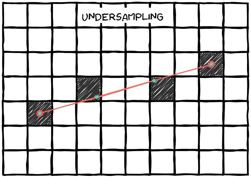
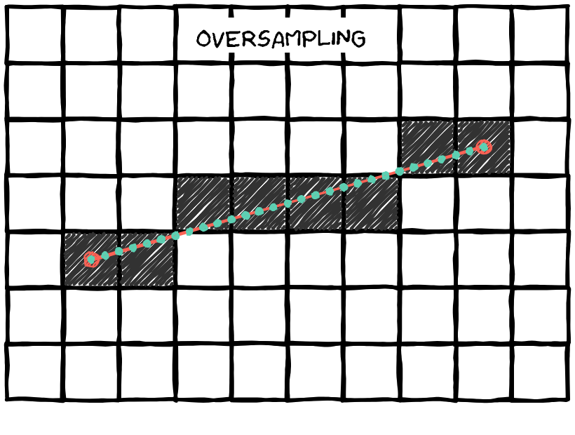
The problem is, we can sample too many points which could result in lot's of unnecessary computations (oversampling); or, we could sample less points but we could skip some pixels and have a line with "holes" (undersampling).
In this interactive animation, you can drag the two red dots and see the rendered line on the pixel screen. You can also adjust the number of sample points.
How do we solve this problem ?
How can we know the minimum number of samples which doesn't skip pixels ?
We could sample one point for every column like this:
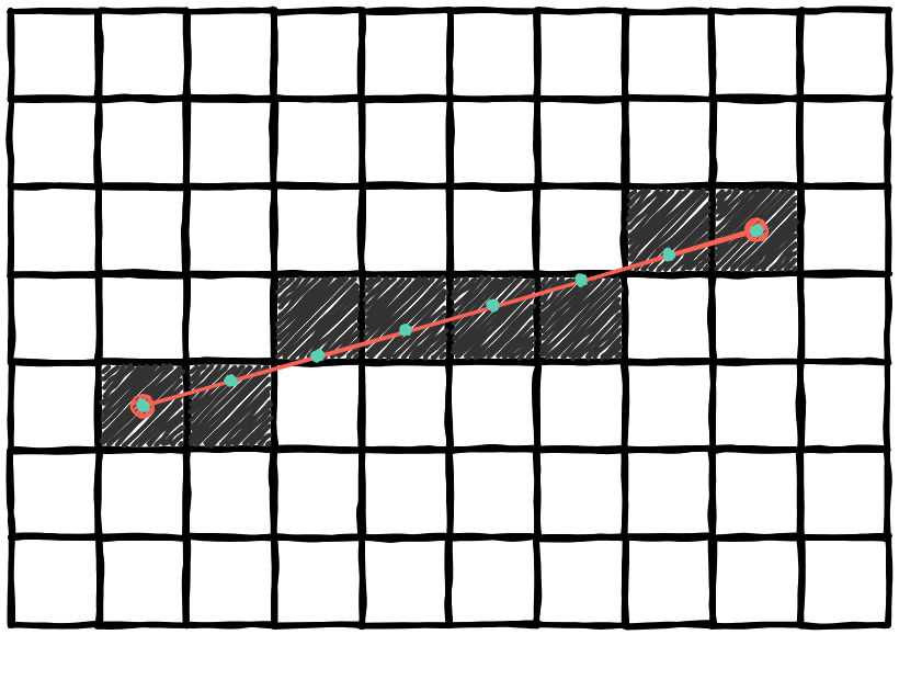
But, it wouldn't work for every line:
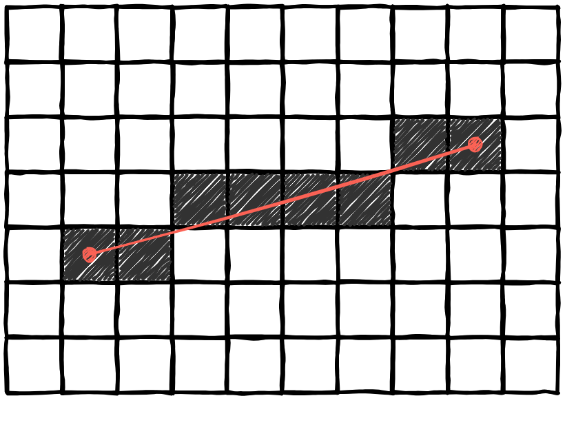
If a line is very steep, between two columns, the gap may be more than 1 pixel.
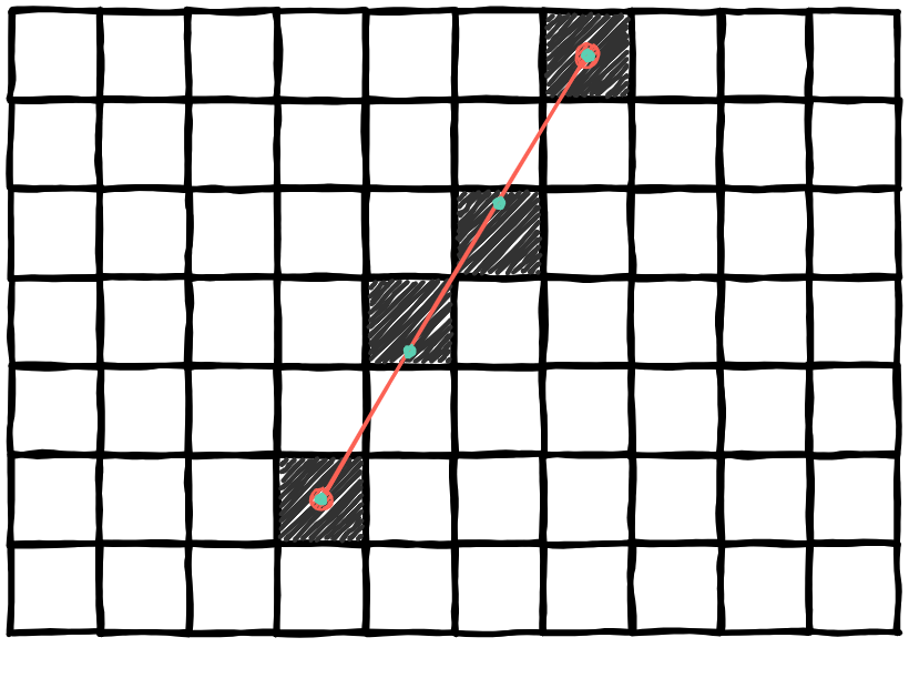
If you take the time to think about it, this method only works when the line has an angle less than 45° with the x-axis. Otherwise, when you go to the next column, the point would be higher than the last by more than 1 pixel.
We can know if the angle and the x-axis is more than 45° when $\lvert \Delta y \rvert > \lvert \Delta x \rvert$, as shown in the drawing bellow.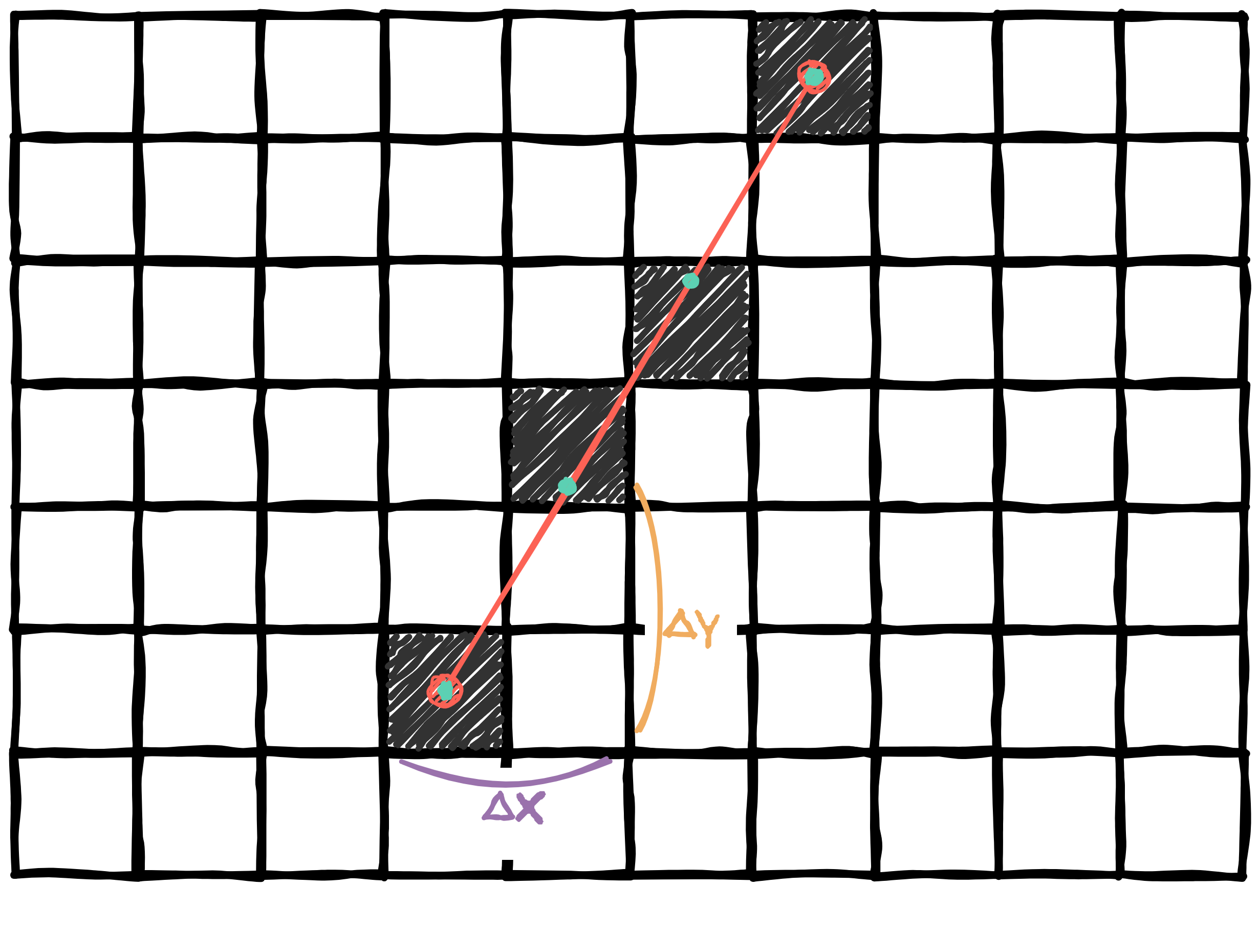
So, if the line is too steep, we can sample every row instead of every column.
How is it implemented in code ?
def line(ax, ay, bx, by):
    dx = ax - bx
    dy = ay - by

    point(ax, ay)
    point(bx, by)

    if abs(dx) >= abs(dy):
        # sample with the columns
        samples = round(abs(dx))
    else:
        # sample with the rows
        samples = round(abs(dy))

    for i in range(0, samples):
        alpha = i / samples

        x = lerp(ax, bx, alpha)
        y = lerp(ay, by, alpha)

        point(x, y)
And so, you've discovered, on your own, Bresenham's line algorithm. Well... almost
Linear interpolation
To understand what "lerp" is, here is an example. You have a ball and it needs to move between two points like this:
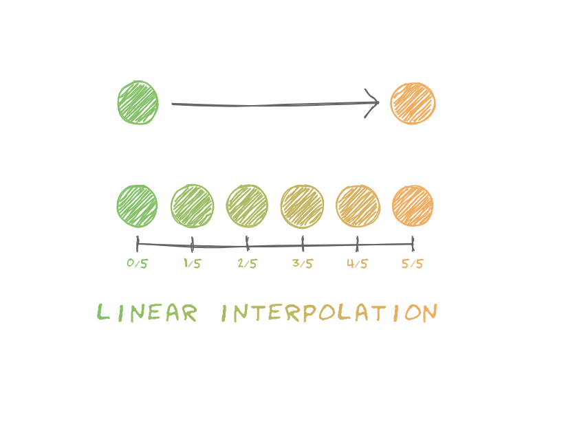
You only have two states of the ball, you don't have the information between those states.
To get this information, you can use "linear interpolation" or "lerp" for short. It allows you to transform smoothly from the first state to the second. This is a function where you give it 3 numbers, $x_s$ (start state), $x_e$ (end state), and a number between 0 and 1 commonly named $t$ or $\alpha$. The $t$ value can be imagined as a "percentage" of the transformation.
Also, the lerp function is defined like this: $lerp(x_s,x_e,t)=x_e t + x_s (1 - t)$.
Here, you can use $x$ and $y$ as the coordinates of the center of the ball, and $r$,$g$, and $b$ to represent the red, green, blue components of the color. So you would have:
$$ x(t) = lerp(x_0, x_1, t)\\y(t) = lerp(y_0, y_1, t)\\ r(t) = lerp(r_0, r_1, t)\\ g(t) = lerp(g_0, g_1, t)\\ b(t) = lerp(b_0, b_1, t)\\ $$
If we apply these rules and make $t$ goes from $0$ to $1$ (repeating indefinitely) and go back to $0$ we get this:
Now, we can go back to Bresenham's line algorithm. Why isn't our algorithm the same as Bresenham's ? It was developed in 1962, and at this time, you could only use integers with a computer. This is the amazing part of Bresenham's algorithm, it works while only using integers. And our algorithm is using decimal numbers. Bresenham's line algorithm use incremental errors. I won't cover this algorithm since, nowadays, most of the time we have access to Floating Point Arithmetic. Also, our algorithm gives back the same results and it is easier to understand.
So, here is an interactive animation to "play" with the algorithm we discovered:
This is the end of this blog post. I hope you'll explore more the amazing world of Mathematics and Computer Science.
Interesting topics to explore:
- Rasterization (I'm working on a part 2 about it)
- 3D shading
- Bezier curves
- Anti-aliasing
Thank you for reading.
Thanks to Grant Sanderson (aka 3Blue1Brown) for inspiring me to make this project.
All of the animation (interactive or not) were created using an open-source tool I made: Manim Web